Linear dependence index

The linear dependence index (LDI) is a measure of the linear dependence of a set of vectors. It is defined as the product of the singular values of the matrix whose columns are the vectors in the set. The LDI provides a quantitative measure of whether a set of vectors is linearly independent or dependent.

Given a matrix \(A \in \mathbb{R}^{d \times k}\), where \(d\) is the dimension of the vectors and \(k\) is the number of vectors, we compute the singular value decomposition (SVD) of the matrix:

\[A = U \Sigma V^T\]

where \(U\) is a \(d \times d\) orthogonal matrix, \(\Sigma\) is a \(d \times k\) diagonal matrix with non-negative entries (the singular values, \(\sigma_i = \Sigma_{ii}\)), and \(V\) is a \(k \times k\) orthogonal matrix. The linear dependence index is then defined as:

\[\text{LDI}_k = \prod_{i=1}^{\min(d, k)} \sigma_i\]

In our case, the matrix \(A\) is the matrix whose columns are \(k\) deviation vectors that evolve according to the linearized dynamics:

\[\frac{dA(t)}{dt} = J(\mathbf{x}(t), t)A(t).\]

To avoid the numerical instability that arises from the exponential divergence of the deviation vectors for chaotic trajectories, we normalize the columns of \(A\) at each time step before computing its SVD.

To illustrate the calculation of the LDI, we are going to consider a 4-dimensional version of the Rössler system, given by:

\[\begin{split}\begin{align*} \dot{x} &= - y - z,\\ \dot{y} &= x + ay + w, \\ \dot{z} &= b + xz, \\ \dot{w} &= -cz + dw, \end{align*}\end{split}\]

with parameters \(a = 0.25\), \(b = 3.0\), \(c = 0.5\), and \(d = 0.05\). This set of parameters yield a hyperchaotic solution, i.e., a trajectory with more than one positive Lyapunov exponent. Let’s visualize that:

from pynamicalsys import ContinuousDynamicalSystem as cds
from pynamicalsys import PlotStyler

ds = cds(model="4d rossler system")
ds.integrator("rk45", atol=1e-15, rtol=1e-15)

# Parameters of the system
a, b, c, d = 0.25, 3.0, 0.5, 0.05
parameters = [a, b, c, d]
ds.set_parameters(parameters)

# Initial condition
u = [-20, 0, 0, 15]

# Total and transient times
total_time = 100000
transient_time = 1000

# Calculate the Lyapunov exponents
lyapunov_exponents = ds.lyapunov(
    u,
    total_time,
    transient_time=transient_time,
    return_history=True
)

# Set the plot style
ps = PlotStyler(fontsize=18)
ps.apply_style()

# Create the figure and axes
fig, ax = plt.subplots(1, 2, sharex=True, figsize=(10, 3))
ps.set_tick_padding(ax[0], pad_x=6)
ps.set_tick_padding(ax[1], pad_x=6)

# Plot each Lyapunov exponent with a different color
colors = ["green", "gold", "blue", "red"]
for i in range(4):
    ax[0].plot(
        lyapunov_exponents[:, 0],
        lyapunov_exponents[:, i + 1],
        color=colors[i],
        label=rf"$\lambda_{i + 1}$")

# Plot the first three in log scale to enphasize that :math:`\lambda_{1,2} > 0`
# and that :math:`\lambda_3 \rightarrow 0`
for i in range(3):
    ax[1].plot(
        lyapunov_exponents[:, 0],
        abs(lyapunov_exponents[:, i + 1]),
        color=colors[i],
        label=rf"$\lambda_{i + 1}$")

# Set the legend, labels, and limits
ax[0].legend(loc="center right", frameon=False, ncol=2)
ax[0].set_ylabel("Lyapunov exponents")
ax[0].set_xlabel("Time")
ax[1].set_xlabel("Time")
ax[0].set_xlim(transient_time, total_time)
ax[1].set_yscale("log")
ax[1].set_xscale("log")

plt.show()

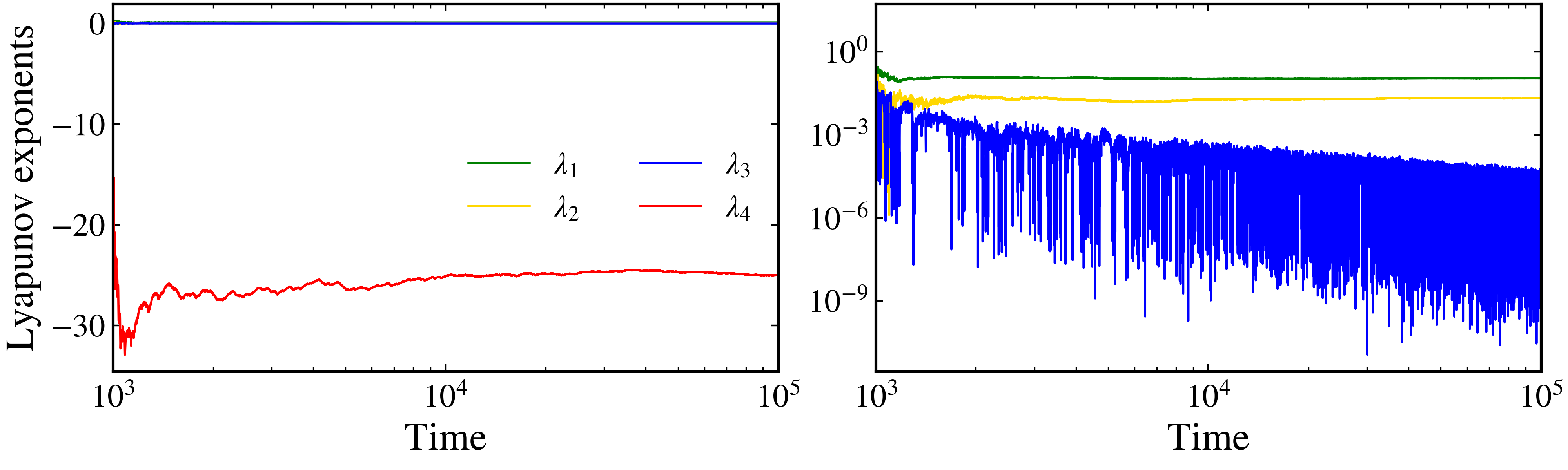
The Lyapunov exponents for the 4D Rössler system.

Let’s then compute the LDI’s using 2, 3, and 4 deviation vectors for the 4-dimensional Rössler system. The LDI is computed using LDI method from the ContinuousDynamicalSystem class:

from pynamicalsys import ContinuousDynamicalSystem as cds

ds = cds(model="4d rossler system")
ds.integrator("rk45", atol=1e-15, rtol=1e-15)

# Parameters of the system
a, b, c, d = 0.25, 3.0, 0.5, 0.05
parameters = [a, b, c, d]
ds.set_parameters(parameters)

# Initial condition
u = [-20, 0, 0, 15]

# Total and transient times
total_time = 2000
transient_time = 1000

# Calculate the LDI's
ldi = []
for k in (2, 3, 4):
    ldi.append(ds.LDI(
        u,
        total_time,
        k,
        parameters=parameters,
        transient_time=transient_time,
        return_history=True)
    )

The LDI method returns a 2D array of shape (samples, 2), where the columns are the times samples where the LDI was calculated and the LDI value itself. We can visualize the behavior of each LDI by plotting it in a log-lin plot:

from pynamicalsys import PlotStyler
import matplotlib.pyplot as plt

# Set the style
ps = PlotStyler(fontsize=18)
ps.apply_style()

# Create the figure and axes
fig, ax = plt.subplots(1, 2, sharey=True, figsize=(10, 3))

# Plot LDI_2 and LDI_3 in the same plot
ax[0].plot(ldi[0][:, 0], ldi[0][:, 1], color="k", label="LDI$_2$")
ax[0].plot(ldi[1][:, 0], ldi[1][:, 1], "r-", label="LDI$_3$")

# Plot LDI_4 in the second plot
ax[1].plot(ldi[2][:, 0], ldi[2][:, 1], "k-")

# Set the labels, limits, legend and titles
ax[0].set_yscale("log")
ax[0].set_ylim(1e-16, 1e1)
ax[0].set_xlabel("Time")
ax[0].set_ylabel("Linear dependence index")
ax[0].set_title("LDI$_2$ and LDI$_3$", fontsize=18)
ax[0].set_xlim(transient_time, ldi[0][-1, 0])
ax[0].legend(loc="upper right", frameon=False)
ax[1].set_xlabel("Time")
ax[1].set_title("LDI$_4$", fontsize=18)
ax[1].set_xlim(transient_time, ldi[2][-1, 0])

plt.show()

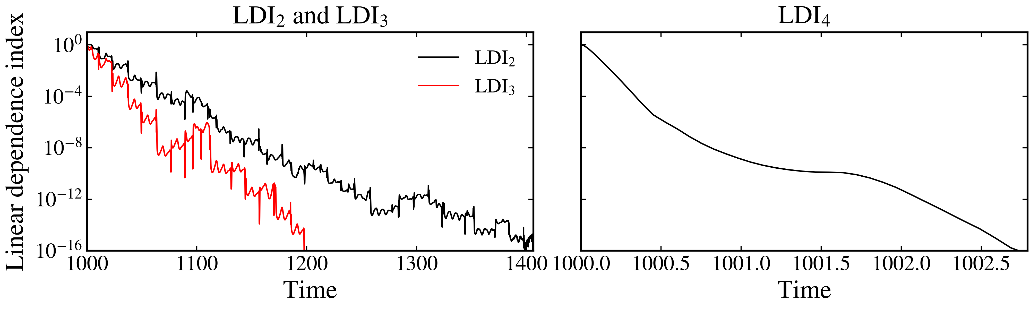
The LDI for \(k = 2\), \(k = 3\), and \(k = 4\).