Generating trajectories

To generate trajectories for a continuous dynamical system, we use the trajectory method of the HamiltonianSystem class. This method allows us to specify the initial condition, parameter values, and total time for the simulation. It is possible to choose between three different integrators: the 2nd order velocity Verlet (VV2), the 4th order Yoshida (SVY4), and the implicit midpoint method (IMP). The first two can only be used for separable Hamiltonians.

Choosing the integrator

To choose the integrator, we use the integrator method of the HamiltonianSystem class. Both VV2 and SVY4 integrators only need the time step, which is set to \(10^{-2}\) by default:

from pynamicalsys import HamiltonianSystem

ds = HamiltonianSystem(model="henon heiles")
ds.integrator("svy4", time_step=0.005)

For the IMP method, it is also possible to specify the tolerance and maximum iterations for the internal root finder:

ds.integrator("imp", time_step=0.005, tol=1e-9, max_iter=10000)

Trajectories and energy conservation

Let’s now generate a trajectory for the Hénon-Heiles system using these tree integrators. We first import all the necessary modules to simulate and visualize the trajectories and instanciante the HamiltonianSystem class:

from pynamicalsys import HamiltonianSystem, PlotStyler
import numpy as np
import matplotlib.pyplot as plt
import seaborn as sns

ds = HamiltonianSystem(model="henon heiles")

Next, we can generate a trajectory by specifying the initial condition, parameters, and total time. The trajectory method returns a Numpy array with shape (N, d + 1), where N is the number of iterations and d is the dimension of the system. The first column corresponds to the time samples at which the trajectory was calculated and the remaing columns correspond to a state variable.

# Total energy of the system
E = 1 / 8

# Total integration time
total_time = 10000

# Initial condition
x = 0
y = 0.1
py = 0
px = np.sqrt(2 * (E - x**2 * y + y**3 / 3) - x**2 - y**2 - py**2)
q = np.array([x, y])
p = np.array([px, py])

# Using VV2 integrator
ds.integrator("vv2", time_step=0.01)

# Generate the trajectory
traj_vv2 = ds.trajectory(q, p, total_time)

# Using SVY4 integrator
ds.integrator("svy4", time_step=0.01)

# Generate the trajectory
traj_svy4 = ds.trajectory(q, p, total_time)

# Using IMP integrator
ds.integrator("imp", time_step=0.01, tol=1e-9, max_iter=1000)

# Generate the trajectory
traj_imp = ds.trajectory(q, p, total_time)

Then we can plot the trajectory:

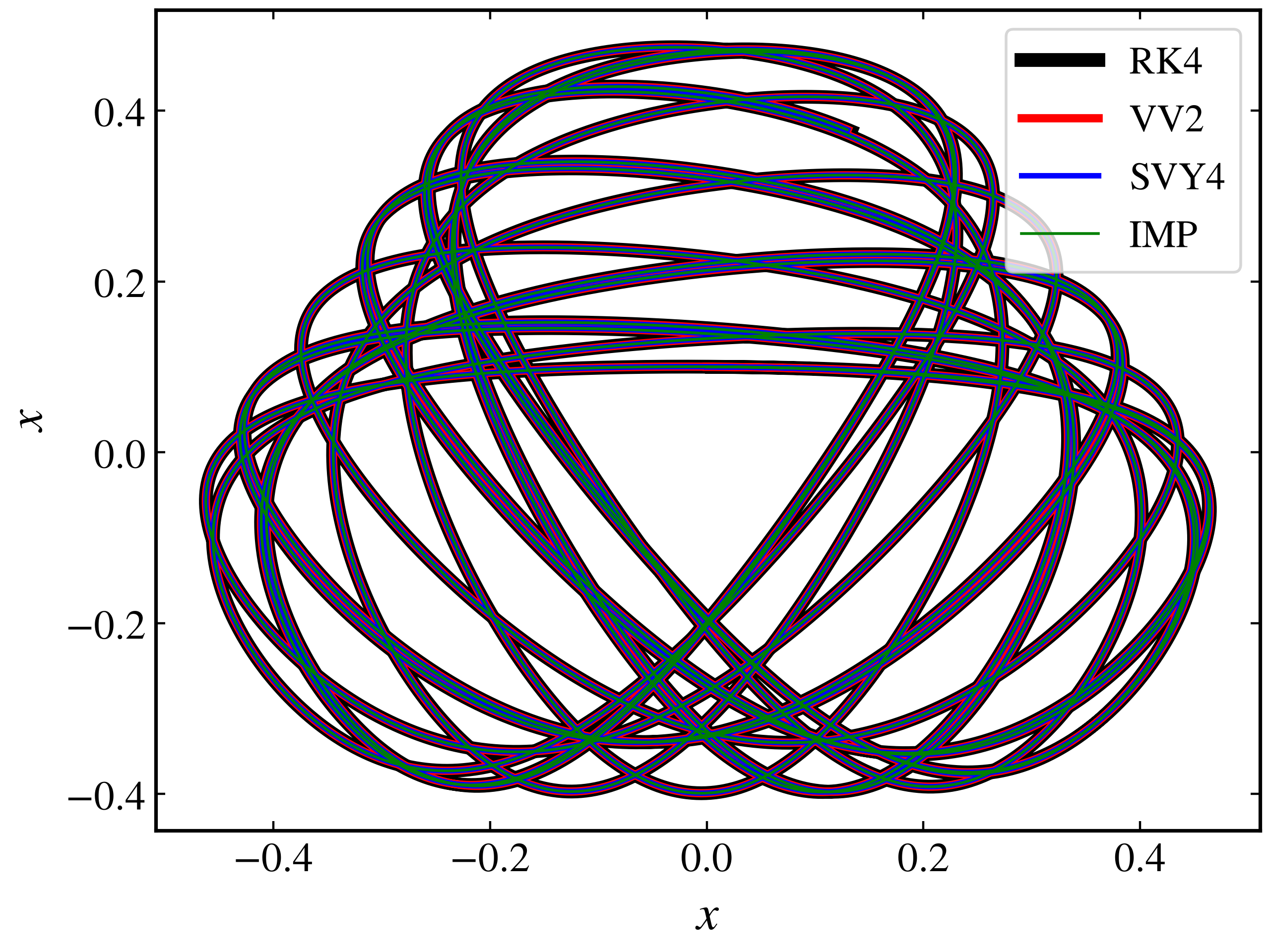
A regular trajectory of the Hénon-Heiles system using four different integrators.

To check the energy drift of each integrator, we calculate the relative energy error:

\[\begin{equation*} E_r = \frac{\left|E(t) - E_0\right|}{E_0}. \end{equation*}\]

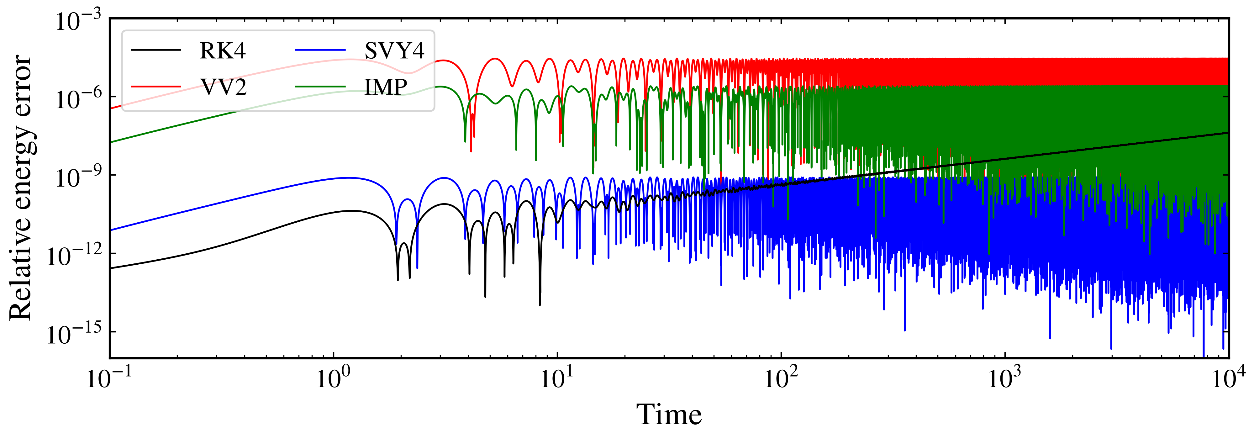
Relative energy error as a function of time of four different integrators.