Recurrence time entropy
A recurrence plot records when a trajectory returns close to a state that it visited previously. This representation was introduced by Eckmann et al. (1987). For a trajectory \(\{\mathbf{x}_i\}_{i=1}^{N}\), the recurrence matrix is
where \(\Theta\) is the Heaviside function, \(\varepsilon\) is the recurrence threshold, and the norm determines the distance between states. A recurrence is recorded when \(R_{ij}=1\).
The zeros between consecutive recurrence points in a column form white vertical lines. Their lengths estimate the recurrence times of the trajectory. If \(P_w(v)\) is the number of white vertical lines of length \(v\), the normalized distribution is
The recurrence time entropy (RTE) is the Shannon entropy of this distribution:
The entropy of a recurrence-period distribution was introduced by Little et al. (2007). Zou et al. (2007) estimated recurrence times from the white vertical lines of recurrence plots, and Sales et al. (2023) used the resulting entropy to detect stickiness and weak chaos in area-preserving maps.
Interpreting RTE
The interpretation is motivated by Slater’s theorem. An irrational rotation on a circle has at most three return times to a connected interval, with the third equal to the sum of the other two. Consequently, periodic motion has a single recurrence time and \(\mathrm{RTE}=0\), while quasiperiodic motion generally produces a small number of recurrence times and a low RTE. Chaotic motion has a broader recurrence-time distribution and typically produces a larger RTE.
For mixed phase spaces, sticky chaotic trajectories temporarily resemble quasiperiodic motion near regular islands. Their RTE can therefore be lower than that of trajectories moving through the chaotic sea but higher than that of regular trajectories. Sales et al. (2023) showed that RTE is strongly positively correlated with the largest Lyapunov exponent for the standard map and that the finite-time RTE distribution can resolve different hierarchical levels of islands around islands.
These statements describe the relative behavior of RTE for a fixed analysis procedure. RTE values depend on the trajectory length, recurrence threshold, distance metric, minimum line length, and scaling of the state variables. They should not be compared across calculations that use incompatible settings.
Choosing the recurrence threshold
The threshold \(\varepsilon\) must be large enough to produce a useful number of recurrences but small enough to preserve local phase-space structure. The recurrence_time_entropy method provides three threshold strategies through threshold_mode:
threshold_mode="std"Interprets
thresholdas a scale multiplying the norm of the componentwise standard-deviation vector. Withthreshold=0.1andstd_metric="supremum", the threshold is \(\varepsilon=0.1\max_j\sigma_j\). This reproduces the choice used by Sales et al. (2023) for the standard map.threshold_mode="direct"Uses
thresholddirectly in the units of the state-space distance. This is useful when a physically meaningful neighborhood size is known.threshold_mode="rr"Chooses \(\varepsilon\) from the quantile of the off-diagonal pairwise distances so that
thresholdspecifies a target recurrence rate. In this mode,thresholdmust lie strictly between zero and one.
For "std" and "direct", threshold must be positive. The deprecated threshold_std option should not be used in new code. Its replacements are threshold_mode="std" and threshold_mode="direct".
The metric option controls distances between trajectory states and accepts "supremum", "euclidean", "manhattan", or a callable. The std_metric option independently controls how the componentwise standard deviations are combined in "std" mode and accepts the same named norms or a callable. The defaults are the supremum norm for both. If the state variables have very different physical scales, normalize them first or choose a metric that accounts for those scales.
For example, the three threshold modes can be selected as follows:
initial_state = [0.05, 0.05]

rte_std = system.recurrence_time_entropy(
    u=initial_state,
    total_time=5_000,
    parameters=[1.5],
    threshold_mode="std",
    threshold=0.1,
    metric="supremum",
    std_metric="supremum",
)

rte_direct = system.recurrence_time_entropy(
    u=initial_state,
    total_time=5_000,
    parameters=[1.5],
    threshold_mode="direct",
    threshold=0.02,
)

rte_rr = system.recurrence_time_entropy(
    u=initial_state,
    total_time=5_000,
    parameters=[1.5],
    threshold_mode="rr",
    threshold=0.05,
)
The minimum accepted white-line length is controlled by lmin and defaults to one. Increasing it removes the shortest recurrence times before the probability distribution and entropy are calculated.
Optional outputs
By default, recurrence_time_entropy returns only the scalar RTE. The method can also return the final state, recurrence matrix, and normalized nonzero white-line distribution. Requested outputs always follow the RTE in that order:
rte, final_state, recurrence_matrix, distribution = system.recurrence_time_entropy(
    u=initial_state,
    total_time=5_000,
    parameters=[1.5],
    threshold_mode="std",
    threshold=0.1,
    return_final_state=True,
    return_recmat=True,
    return_p=True,
)
The recurrence matrix contains \(N^2\) entries, so both its construction and storage become expensive for long trajectories. Use only the trajectory length needed to resolve the recurrence-time distribution, and request return_recmat=True only when the matrix itself is needed.
Comparing parameter values
The following example keeps the same ensemble of random initial conditions and compares the standard map at \(k=0.9\), \(k=1.5\), and \(k=3.6\). For each trajectory, the recurrence threshold is ten percent of the supremum norm of its standard-deviation vector:
import numpy as np
import matplotlib.pyplot as plt
from pynamicalsys import DiscreteDynamicalSystem as dds, PlotStyler

system = dds(model="standard map")

num_initial_conditions = 250
np.random.seed(0)
x_initial = np.random.uniform(0.0, 1.0, num_initial_conditions)
y_initial = np.random.uniform(0.0, 1.0, num_initial_conditions)
initial_states = np.column_stack((x_initial, y_initial))
parameter_values = [0.9, 1.5, 3.6]
total_time = 10_000

rte_values = np.empty((len(parameter_values), num_initial_conditions))
trajectories = np.empty(
    (len(parameter_values), num_initial_conditions, total_time, 2)
)
for i, k in enumerate(parameter_values):
    for j, initial_state in enumerate(initial_states):
        rte_values[i, j] = system.recurrence_time_entropy(
            u=initial_state,
            total_time=total_time,
            parameters=[k],
            threshold_mode="std",
            threshold=0.1,
            metric="supremum",
            std_metric="supremum",
        )

    trajectories[i] = system.trajectory(
        u=initial_states,
        total_time=total_time,
        parameters=[k],
    ).reshape(num_initial_conditions, total_time, 2)
Plot the trajectories and assign every point the RTE of the initial condition that generated it:
ps = PlotStyler()
ps.apply_style()
fig, ax = plt.subplots(1, 3, figsize=(12, 4), sharex=True, sharey=True)
for i, k in enumerate(parameter_values):
    trajectory_rte = np.repeat(rte_values[i], total_time)
    points = ax[i].scatter(
        trajectories[i, :, :, 0].ravel(),
        trajectories[i, :, :, 1].ravel(),
        c=trajectory_rte,
        s=0.05,
        edgecolor="none",
        cmap="nipy_spectral",
        vmin=0.0,
        vmax=rte_values[i].max(),
    )
    fig.colorbar(
        points,
        ax=ax[i],
        label=rf"RTE with $k={k:.1f}$",
        location="top",
        aspect=40,
        pad=0.01,
    )
    ax[i].set_xlim(0.0, 1.0)
    ax[i].set_ylim(0.0, 1.0)
    ax[i].set_xlabel("$x$")
ax[0].set_ylabel("$y$")
fig.tight_layout()
plt.show()
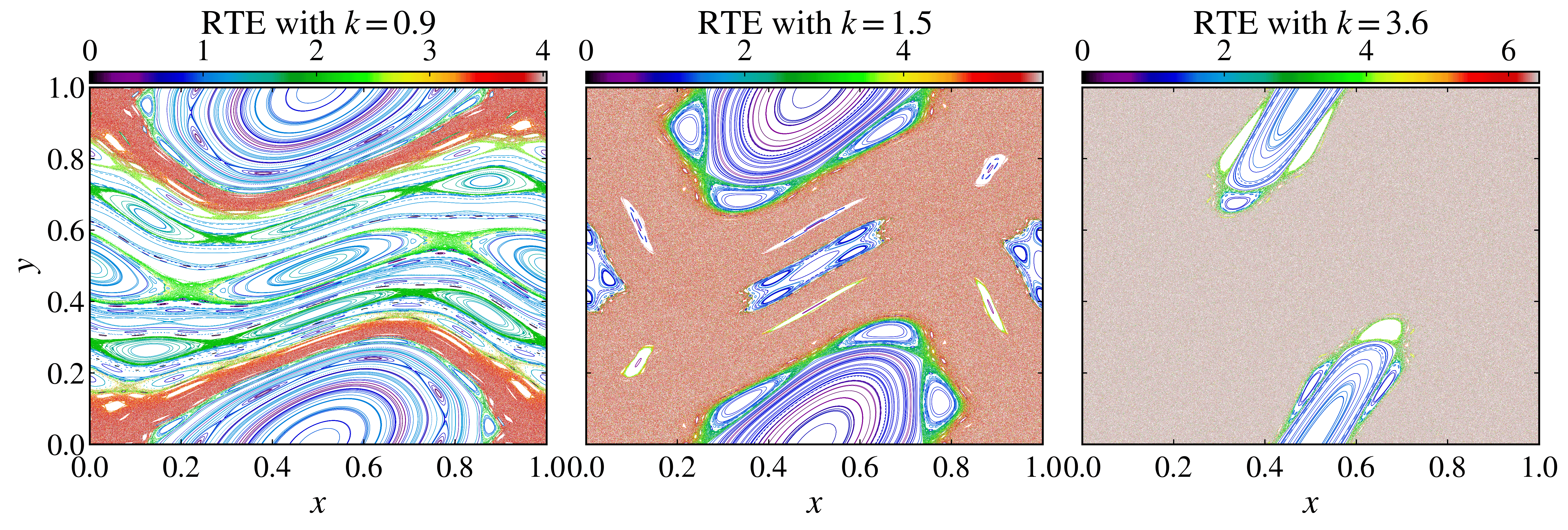
Standard-map trajectories colored by their recurrence time entropy for three values of \(k\).
At \(k=0.9\), invariant curves occupy much of the phase space. At \(k=1.5\), the chaotic sea coexists with prominent regular islands and sticky layers. At \(k=3.6\), the chaotic component is larger while smaller regular structures remain. Within each panel, low RTE values identify trajectories with a narrow recurrence-time distribution and high values identify trajectories with a broader distribution.
Finite-time RTE
Use finite_time_recurrence_time_entropy to follow changes along one trajectory. The method divides total_time into consecutive non-overlapping windows of length finite_time and returns one RTE value per complete window. Any remainder shorter than finite_time is not used.
finite_rte, phase_space_points = system.finite_time_recurrence_time_entropy(
    u=[0.05, 0.05],
    total_time=100_000,
    finite_time=200,
    parameters=[1.5],
    return_points=True,
    threshold_mode="std",
    threshold=0.1,
)
When return_points=True, phase_space_points[i] is the state at the beginning of the window that produced finite_rte[i]. A multimodal finite-time RTE distribution can reveal transitions between the chaotic sea and sticky layers, but the locations of its modes depend on the window length and threshold settings.
References
J.-P. Eckmann, S. O. Kamphorst, and D. Ruelle, Recurrence plots of dynamical systems, Europhysics Letters 4, 973-977 (1987).
M. A. Little, P. E. McSharry, S. J. Roberts, D. A. E. Costello, and I. M. Moroz, Exploiting nonlinear recurrence and fractal scaling properties for voice disorder detection, BioMedical Engineering OnLine 6, 23 (2007).
Y. Zou, M. Thiel, M. C. Romano, and J. Kurths, Characterization of stickiness by means of recurrence, Chaos 17, 043101 (2007).
M. R. Sales, M. Mugnaine, J. D. Szezech Jr., R. L. Viana, I. L. Caldas, N. Marwan, and J. Kurths, Stickiness and recurrence plots: An entropy-based approach, Chaos 33, 033140 (2023).
N. B. Slater, The distribution of the integers N for which {θN} < φ, Mathematical Proceedings of the Cambridge Philosophical Society 46, 525-534 (1950).
N. B. Slater, Gaps and steps for the sequence nθ mod 1, Mathematical Proceedings of the Cambridge Philosophical Society 63, 1115-1123 (1967).