Transport and diffusion
Transport describes how trajectories move through phase space and how an ensemble of initial conditions spreads. In an area-preserving map, invariant curves can block global motion and chaotic trajectories can remain trapped near regular islands for long intervals. The resulting spreading need not follow the linear growth expected for normal diffusion. The standard map has long served as a fundamental model for studying these mechanisms, as reviewed by Chirikov (1979).
Two versions of the standard map are used on this page. The bounded standard map is used to examine recurrence times. The unbounded standard map keeps the angle modulo one but allows the action to grow without bounds, making it suitable for measuring diffusion.
import numpy as np
import matplotlib.pyplot as plt
from pynamicalsys import DiscreteDynamicalSystem as dds, PlotStyler
Diffusion of an ensemble
When the action is unbounded, an ensemble of initial conditions can spread indefinitely. The central quantity is the mean squared displacement of the action,
where the average is taken over the ensemble. Normal diffusion satisfies \(\mathrm{MSD}(n)\sim 2Dn\), while anomalous diffusion follows \(\mathrm{MSD}(n)\sim n^\gamma\) with \(\gamma\neq1\). Accelerator modes can produce ballistic motion with \(\gamma=2\) and strongly influence the surrounding chaotic transport, as discussed by Karney et al. (1982) and Karney (1983).
The mean_squared_displacement method follows an ensemble and measures the displacement along the coordinate selected by axis. Here, 900 initial conditions are distributed across the unit square and the action is measured with axis=1:
system = dds(model="unbounded standard map")

rng = np.random.default_rng(0)
num_ic = 30 * 30
x0 = np.random.uniform(0, 1, num_ic)
y0 = np.random.uniform(0, 1, num_ic)
initial_conditions = np.column_stack([x0, y0])
total_time = int(1e6)

k1 = 5.0
system.set_parameters([k1])
msd_normal = system.mean_squared_displacement(initial_conditions, total_time, axis=1)

k2 = 6.75
system.set_parameters([k2])
msd_anomalous = system.mean_squared_displacement(initial_conditions, total_time, axis=1)
Each call returns a one-dimensional array of length total_time, containing the mean squared displacement from iteration 1 through total_time. At \(k=5.0\), the growth is approximately linear. At \(k=6.75\), an accelerator mode produces nearly ballistic spreading.
time = np.arange(1, total_time + 1)
ps = PlotStyler()
ps.apply_style()
fig, ax = plt.subplots(figsize=(6, 4))
ax.loglog(time, msd_normal, "b", label=f"$k = {k1}$", lw=1.5)
ax.loglog(time, msd_anomalous, "r", label=f"$k = {k2}$", lw=1.5)
ax.loglog(time, 3 * msd_normal[0] * time, "k--", lw=1, label=r"slope $1$")
ax.loglog(time, 0.03 * time**2, "k:", lw=1, label=r"slope $2$")
ax.set_xlabel("Iteration $n$")
ax.set_ylabel(r"$\mathrm{MSD}(n)$")
ax.set_ylim(1e2, 1e12)
ax.set_xlim(5e2, total_time)
ax.legend(frameon=False)
fig.tight_layout()
plt.savefig(
    f"{path_figures}/standard_map_diffusion_msd.png", dpi=400, bbox_inches="tight"
)
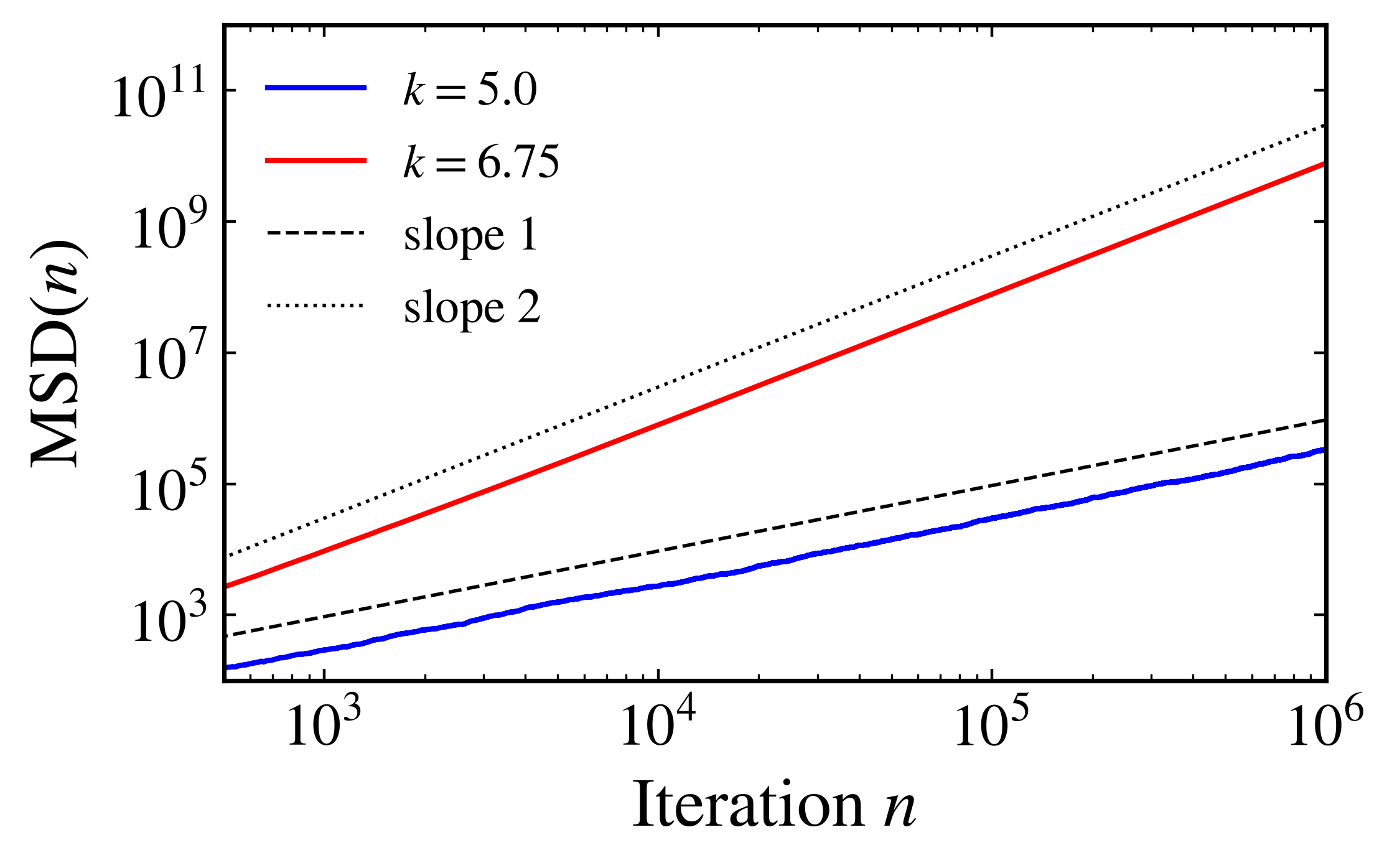
Mean squared displacement of the action for the unbounded standard map. The curve for \(k=5.0\) follows the slope-one reference for normal diffusion, while the curve for \(k=6.75\) approaches the slope-two reference for ballistic transport.
Diffusion coefficient
For normal diffusion, the diffusion_coefficient method estimates \(D\) from the final ensemble displacement through the Einstein relation \(D\approx\mathrm{MSD}(N)/(2N)\). Analytical corrections to the random-phase approximation for the Chirikov-Taylor map were developed by Rechester et al. (1981).
For the normalization used by pynamicalsys, uncorrelated angle kicks have variance \(k^2/(8\pi^2)\), giving the random-phase estimate
The measured coefficient at \(k=5.0\) is close to this estimate:
system.set_parameters([5.0])
D = system.diffusion_coefficient(initial_conditions, total_time, axis=1)
print("measured D:", float(D))
print("random-phase D:", 5.0**2 / (16 * np.pi**2))
measured D: 0.1575283354658878
random-phase D: 0.15831434944115277
A single diffusion coefficient is meaningful only when the mean squared displacement is asymptotically linear. For anomalous transport, \(\mathrm{MSD}(N)/(2N)\) depends on the observation time and the spreading must instead be characterized by the exponent \(\gamma\).
Summaries of the ensemble
Several methods summarize the same ensemble along the selected axis and can optionally record only chosen sample_times. The average_in_time method returns the ensemble mean of the coordinate at each sampled time. The cumulative_average method returns its cumulative time average. The root_mean_squared method gives the root mean square accumulated over time, which measures the typical width of the ensemble.
system.set_parameters([5.0])
mean = system.average_in_time(initial_conditions, total_time, axis=1)
rms = system.root_mean_squared(initial_conditions, total_time, axis=1)
The ensemble_time_average method returns one centered time average per trajectory. Each trajectory average has the ensemble mean subtracted, so the returned values quantify trajectory-to-trajectory fluctuations around the ensemble average.
eta = system.ensemble_time_average(initial_conditions, total_time, axis=1)
print(eta.shape, round(float(eta.mean()), 3), round(float(eta.std()), 3))
(5000,) 0.0 10.292
Recurrence times and stickiness
For a measure-preserving map on a bounded phase space, the Poincaré recurrence theorem guarantees that almost every initial condition eventually returns arbitrarily close to its starting point. In a mixed phase space, trajectories can remain close to regular islands for long intervals before returning. These trapping episodes generate long-time correlations and heavy recurrence-time tails, as studied for the standard map by Chirikov and Shepelyansky (1999).
The recurrence_times method records the number of iterations between successive entries into a hypercube centered on the initial state. The argument eps gives the side length of this recurrence neighborhood. An optional transient_time can be used to evolve the initial condition before defining its center.
system = dds(model="standard map")
system.set_parameters([1.5])
times = system.recurrence_times([0.2, 0.02], 1_000_000_000, eps=0.02)
print(times.size, times.min(), times.max(), times.mean())
561463 7.0 475852.0 1781.0521405684792
The observed return times range from 7 iterations to more than 475,000 iterations. Their mean is much smaller than their maximum, indicating a broad distribution generated by long trapping episodes.
counts, edges = np.histogram(
    times, bins=np.logspace(0, np.log10(times.max()), 100), density=True
)
centers = np.sqrt(edges[:-1] * edges[1:])

ps = PlotStyler()
ps.apply_style()
fig, ax = plt.subplots(figsize=(6, 4))
ax.loglog(centers, counts, "o", markersize=4)
ax.set_xlabel(r"Recurrence time $\tau$")
ax.set_ylabel(r"$P(\tau)$")
ax.set_xlim(times.min(), times.max())
fig.tight_layout()
plt.savefig(
    f"{path_figures}/standard_map_recurrence_times.png", dpi=400, bbox_inches="tight"
)

Recurrence-time distribution for the standard map with \(k=1.5\). The long tail reflects trapping near regular structures in the mixed phase space.
Recurrence times measure the intervals between visits to a neighborhood. The recurrence time entropy instead measures the diversity of recurrence periods obtained from a recurrence plot, so the two quantities provide complementary descriptions of recurrent dynamics.
References
B. V. Chirikov, A universal instability of many-dimensional oscillator systems, Physics Reports 52, 263-379 (1979).
A. B. Rechester, M. N. Rosenbluth, and R. B. White, Fourier-space paths applied to the calculation of diffusion for the Chirikov-Taylor model, Physical Review A 23, 2664-2672 (1981).
C. F. F. Karney, A. B. Rechester, and R. B. White, Effect of noise on the standard mapping, Physica D 4, 425-438 (1982).
C. F. F. Karney, Long-time correlations in the stochastic regime, Physica D 8, 360-380 (1983).
B. V. Chirikov and D. L. Shepelyansky, Asymptotic statistics of Poincaré recurrences in Hamiltonian systems with divided phase space, Physical Review Letters 82, 528-531 (1999).